Optimization of the Booth Function with Differential Evolution

Source: https://www.mdpi.com/journal/applsci/special_issues/Evolutionary_Computation

Introduction to Differential Evolution (DE)

Differential Evolution is a Stochastic Direct Search and Global Optimization algorithm. This was introduced by Storn and Price during 1995/ 1996 and developed to optimize real parameters of real-valued functions.

Fig. 1. Outline of the DE algorithm.

Fig. 1. illustrates the outline of the basic DE algorithm.

Booth Function

Fig. 2. Booth Function

As per the Fig. 2. the Booth Function is defined on a 2-dimentional space and the function has one global minimum at: f(x) = 0 at x = (1,3). This is evaluated on the square xi ∈ [−10, 10] for all i = 1, 2.

Optimization of Booth Function with DE

Here the following steps are followed.

1: Begin 
2: Generate random population of n individuals 
3: Define the fitness function f(X) 
4: Determine the fitness of i th individual Xi via f(Xi) 
5: while End condition do 
6: for Each individual i do 
7: Choose 3 numbers a, b and c, that is 1 ≤ a, b, c ≤ n and 
a != b !=c != i and perform Mutation
8: Generate next generation from Selection and Crossover
9: end for 
10: end while 
11: Pick the agent from the population that has the highest fitness or lowest cost and return it as the best found candidate solution. 12: End

The following describes the algorithm in detail with MATLAB examples.

1. Initially need to create a random set of solutions (base vector - 10*2) called population between -10 and 10. Here n is the population size (n=10).

2. Define the fitness function as,

f(x) =( x1 + 2*x2 - 7)^2 + (2*x1 + x2 - 5)^2

The following steps will be iterated up to 300 steps.

3. Apply the Mutation operation

This creates the donor vector by adding the weighted difference between two population members at random to a third member in each iteration as follows.

v = a + F(b − c) 1 ≤ a, b, c ≤ 10 and a !=b != c != it and 0 ≤ F ≤ 1.

Here a is the it th element of the base vector.

4. Apply Crossover operation

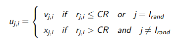
This returns a vector called trail vector by considering the following equation. Here u-trail vector, x-base vector (target vector), v-donor vector, CR-recombination probability (0.5), Irand-an integer random number between (1, dimension).

5. Apply Selection operation

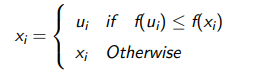
The target vector is compared with the trial vector and the one with the lowest fitness value is selected for the next generation (minimization) as follows.

After considering the selection operation, MSE (mean squared error) is calculated for the itr th step.

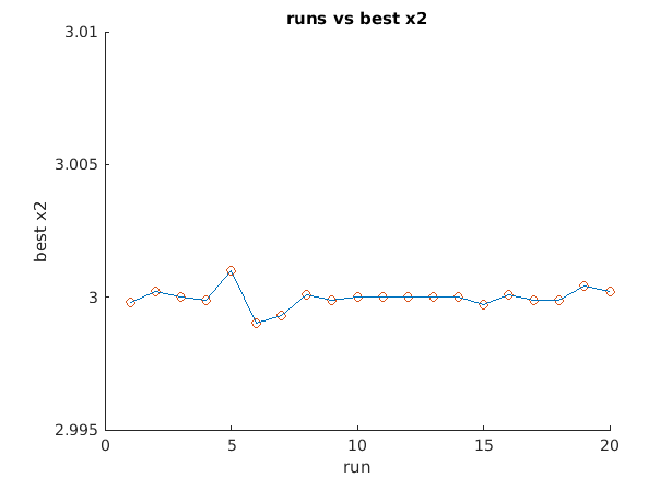
6. Get the best fit at a run

Here find the best fitness value and parameters (x1, x2) of the population at itr th step.

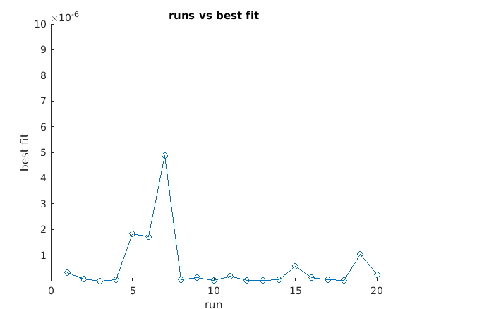
best_at_run(ch) finds the best x1, x2, and fitness value at the i th run.

The following defines the main function.

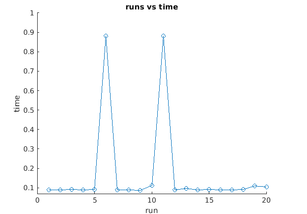
Results

Best fit and corresponding X1 and X2 of this run, 
Best fit: 2.4168e-07 
X1: 0.99979 
X2: 3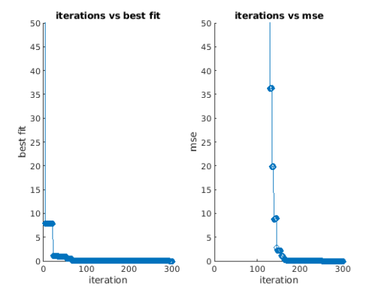

Fig. 3. MSE vs Iterations

Fig. 4. Best Fit vs Runs

Fig. 5. Best X1 vs Runs

Fig. 6. Best X2 vs Runs

Fig. 7. Time vs Runs

Find the work at:

GitHub - HasiniSandunika/Differential-Evolution-with-Booth-Function: Optimization(minimization) of…

References

Evolutionary computation - Wikipedia

Differential evolution - Wikipedia

Booth Function